Longitudinal Analysis

Longitudinal Analysis with Qiime2

There is a lot you can do:

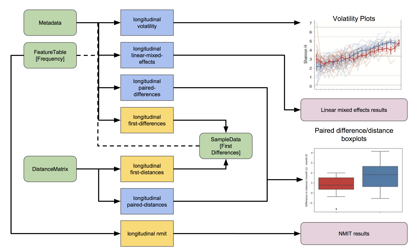
To use the q2-longitudinal plugin, you need a repeated measures sample in which the same site or individual is sampled over time. In the decomp tutorial, samples from each donor were collected over accumulated degree days (ADD), so we can use this tool to understand how the microbiome changed during these periods. Much of these analyses can be done with alpha or beta diversity. For the sake of time, we will focus on just beta diversity.

Let's open up our unweighted UniFrac emperor plot again to help visualize the analysis that we are about to do. Color the samples by host_subject_id. Click on the animations tab and select days add_0c for the gradient and host_subject_id as the trajectory. Then, click the play button and observe. You can adjust the speed to observe changes in beta diversity at a slower pace.

We can see visual changes in beta diversity over time, but this wouldn't be very useful for reporting in a manuscript. Let's look at longitudinal differences with beta diversity so we can start associating numbers and p-values with what we see.

We want to look at how samples from an individual donor change along principal coordinates. So, we will construct a volatility plot which will let us track the beta diversity changes over time within an individual. Volatility refers to the temporal stability of a metric over time and between subjects.

This command is a little different than those we've used before because the parameters we are naming can actually be changed in the visualization. That's why they are called the "defaults". Also, note that we are using the output of the core metrics for this analysis.

PCoA-Based Volatility

First we need to set up and move into the longitudinal directory.

# move back into the decomp_tutorial
cd /scratch/alpine/$USER/decomp_tutorial

# make a longitudinal directory
mkdir longitudinal

# Move into the longitudinal directory
cd longitudinal

Track the position of samples along a PCoA axis over time:

qiime longitudinal volatility \
--m-metadata-file ../metadata/metadata.txt \
--m-metadata-file ../core_metrics/weighted_unifrac_pcoa_results.qza \
--p-state-column add_0c \
--p-individual-id-column host_subject_id \
--p-default-group-column 'sample_type' \
--p-default-metric 'Axis 2' \
--o-visualization pc_vol_sample_type.qzv

Interpreting Volatility Plots

The volatility plot shows how each individual's community composition (summarized by a single PCoA axis) changes over time. Trajectories that converge or diverge between groups suggest temporal differences in community dynamics.

• Once you have an overview of each axis, you can do linear mixed effects models with the axis of interest as the response variable in R. I will usually test the first 3 axes in R for my variables of interest.

First Distances

Calculate Change from Baseline

Another method is to do a distance-based analysis using the first-distances method. In this analysis, we test the hypothesis that microbial community composition changes over accumulated degree days (ADD), measured as the distance from each sample type’s baseline time point (ADD = 0). By specifying a baseline (--p-baseline 0), all subsequent time points are compared back to that fixed reference, allowing us to quantify how much each community diverges from its starting composition over time.

The state column (add_0c) represents accumulated degree days (time), and the individual-id-column (host_subject_id_sample_type) links repeated measures from the same sample type (soil or skin, facility) across time. If the baseline parameter were omitted, the analysis would instead evaluate change between successive time points (i.e., rate of change rather than deviation from the initial state).

Calculate the distance of each sample from its own baseline (ADD = 0) using weighted UniFrac:

qiime longitudinal first-distances \
--i-distance-matrix ../core_metrics/weighted_unifrac_distance_matrix.qza \
--m-metadata-file ../metadata/metadata.txt \
--p-state-column add_0c \
--p-individual-id-column host_subject_id_sample_type \
--p-baseline 0 \
--o-first-distances from_first_wunifrac.qza

Visualize Distance from Baseline

We can again use a volatility analysis to visualize the change in beta diversity based on distance.

qiime longitudinal volatility \
--m-metadata-file ../metadata/metadata.txt \
--m-metadata-file from_first_wunifrac.qza \
--p-state-column add_0c \
--p-individual-id-column host_subject_id \
--p-default-metric Distance \
--p-default-group-column 'sample_type' \
--o-visualization from_first_wunifrac_vol.qzv

Looking at this plot, does one soil type change more over time than the other? What about by facility?

Note: this analysis can also be performed on alpha diversity metrics like Shannon and observed features. From the command above, replace from_first_unifrac.qza file with an alpha diversity file (shannon.qza) and replace the "Distance" metric with "shannon".

Linear Mixed Effects Model

Beta Diversity

Next, we can do a statistical test with a Linear Mixed Effects model. This will let us know if there is a relationship between a dependent variable (diversity) and one or more independent variables, such as accumulated degree days, sample type, facility, etc within the repeated measures.

Since we are interested in the change in distance from the initial time point, we use Distance for --p-metric.

Test whether the distance from baseline changes significantly over time, accounting for facility and sample type:

qiime longitudinal linear-mixed-effects \
--m-metadata-file ../metadata/metadata.txt \
--m-metadata-file from_first_wunifrac.qza \
--p-state-column add_0c \
--p-individual-id-column host_subject_id \
--p-formula "Distance ~ add_0c + facility + sample_type" \
--o-visualization from_first_wunifrac_lme_formula.qzv

There is a new line here, --p-group-columns. While our main question centers around whether accumulated degree day and facility affects the longitudinal change in the microbial community, we also know that sample type plays a large role in shaping the microbial community as well. By including this line, we can account for all of these things "to test whether microbial communities diverge from baseline over accumulated degree days, while controlling for variation due to facility and sample type."

Let's look at this output in q2view now. Here, is there a significant association between the sample type and temporal change? What about facility? If you need a review from a statistics class to understand what the model outputs mean, the table below may help, but this video may also help (play from about 14 min to 20 min): https://www.youtube.com/watch?v=NIGbYdGErLw&list=PLbVDKwGpb3XmvnTrU40zHRT7NZWWVNUpt&index=23

Alpha Diversity Volatility

Track Shannon entropy over time:

qiime longitudinal volatility \
--m-metadata-file ../metadata/metadata.txt \
--m-metadata-file ../core_metrics/shannon_vector.qza \
--p-default-metric shannon_entropy \
--p-default-group-column sample_type \
--p-state-column add_0c \
--p-individual-id-column host_subject_id \
--o-visualization sample_type_shannon_volatility.qzv

Linear Mixed Effects Model

Alpha Diversity

Test whether Shannon entropy changes significantly over time:

qiime longitudinal linear-mixed-effects \
--m-metadata-file ../metadata/metadata.txt \
--m-metadata-file ../core_metrics/shannon_vector.qza \
--p-state-column add_0c \
--p-individual-id-column host_subject_id \
--p-formula "shannon_entropy ~ add_0c + facility + sample_type" \
--o-visualization shannon_lme_formula.qzv

When is time to move your longitudinal analysis outside of Qiime2?

Here are some R packages that are useful for downstream longitudinal analysis.

Linear Mixed Effects Models (lme4) - Fit linear and generalized linear mixed-effects models.

• Can model interactions

• More flexible than the Qiime2 plugin

Estimating Marginal Means (emmeans)

• Compare treatment groups at specific timepoints

• Adjust for covariates like age

• Interpret interactions (e.g., treatment × time)

• Generate adjusted pairwise comparisons with multiple-testing correction

ANCOM-BC2

• Adjust for covariates (like age)

MaAsLin2

• Enables multivariable association testing with fixed and random effects

Outputs

File	Type	Description
pc_vol_sample_type.qzv	Visualization	PCoA-based volatility by sample type
from_first_wunifrac.qza	Artifact	Distance from baseline per sample
from_first_wunifrac_vol.qzv	Visualization	Volatility of distance from baseline
from_first_wunifrac_lme_formula.qzv	Visualization	LME model for beta diversity change
sample_type_shannon_volatility.qzv	Visualization	Shannon entropy volatility
shannon_lme_formula.qzv	Visualization	LME model for Shannon entropy change

Next: Getting Data Into R