Rarefaction

Alpha Rarefaction

Now that we have our tree and we are ready to start looking at the diversity of our samples, we need to normalize first. Rarefying as an option for normalizing your data. As a reminder, we do this because the number of reads differs between samples and this can be unfair when you are doing any statistical analysis between samples.

The command below shows one tool we can use to determine where to rarefy. The plot we are generating subsamples our feature table at different depths and calculates the alpha diversity at each of these. We are looking for the point when the graphs level off and before we start losing lots of real samples, which suggests that at that point we are not gaining any more diversity by adding more sequences. Ideally, we would rarefy at a level where all of the samples have leveled off, though this is not always possible.

Choosing a Max Depth

Set --p-max-depth to approximately the 95^th percentile of your per-sample read counts, which you can identify in the table_dada2_visual_summary.qzv summary from the previous step. Setting it too high wastes computation; too low and your curves may not plateau.

Filtering out controls

Before we do alpha rarefaction we need to filter the control samples out

# Move out of the taxaplot directory into the decomp tutorial 
cd /scratch/alpine/$USER/decomp_tutorial

Now in the decomp tutorial directory run the filtering command

qiime feature-table filter-samples \
--i-table dada2/table_nomitochloro.qza \
--m-metadata-file metadata/metadata.txt \
--p-where "NOT [sample_type] IN ('control') " \
--o-filtered-table dada2/table_nomitochloro_nocontrol.qza

Visuzalize the table, so that we can see the range of sequencing depths across samples

qiime feature-table summarize \
--i-table dada2/table_nomitochloro_nocontrol.qza \
--o-feature-frequencies dada2/feature-frequencies-nomitochloro_nocontrol.qza \
--o-sample-frequencies dada2/sample-frequencies-nomitochloro_nocontrol.qza \
--o-summary dada2/table_nomitochloro_nocontrol.qzv

Generate an Alpha Rarefaction Curve

This command calculates multiple alpha diversity metrics (Faith's PD, observed features, Shannon entropy) at rarefaction depths ranging from 1 to --p-max-depth and plots them as curves. You should choose a --p-max-depth that is just a little bit lower in number than the sample with the most amount of sequences.

Now lets generate an alpha rarefaction plot

# Make the alpha rarefaction directory
mkdir alpha_rarefaction

# Move into the alpha rarefaction directory
cd alpha_rarefaction

qiime diversity alpha-rarefaction \

--i-table ../dada2/table_nomitochloro_nocontrol.qza \

--m-metadata-file ../metadata/metadata.txt \

--p-max-depth \

--o-visualization alpha_rarefaction_curves.qzv

Hint Params

Check →

Open table_nomitochloro.qzv from the previous step. In the interactive table summary, find the value around the 95th percentile of per-sample read counts. Setting max depth too low truncates the curves before they plateau; too high wastes computation.

--p-max-depth, Maximum rarefaction depth (integer). The command calculates diversity at multiple depths from 1 to this value and plots them as curves. Should be approximately the 95th percentile of per-sample read counts from your table summary.

An example rarefaction curve.

• Where the x-axis is the sequencing depth

• Where the y-axis is alpha diveristy or the number of types of microbes per sample.

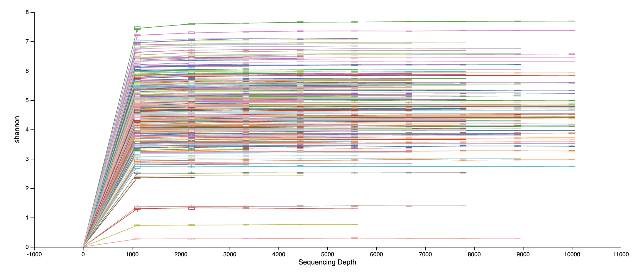
The visualization file will display two plots. The upper plot will display the alpha diversity (observed features or shannon) as a function of the sampling depth. This is used to determine whether the richness or evenness has saturated based on the sampling depth. The rarefaction curve should “level out” as you approach the maximum sampling depth.

The second plot shows the number of samples in each metadata category group at each sampling depth. This is useful to determine the sampling depth where samples are lost, and whether this may be biased by metadata column group values.

Interpreting the Curves

Open alpha_rarefaction_curves.qzv in QIIME2 View and look for the depth where diversity metrics plateau, this is where additional reads no longer add new diversity information.

Choosing a Rarefaction Depth Reset

Identified the plateau depth for all metrics Observed features and Shannon entropy should all stabilize Checked how many samples fall below the chosen depthSamples below this threshold will be excluded from diversity analyses Balanced depth vs. sample retentionDeeper depth retains more reads per sample but drops more samples Confirmed rarefaction depth of 5000 readsUsed in the core metrics step for this workshop dataset

Workshop Rarefaction Depth (the number used in a later analysis step - Core Metrics)

For this dataset, after we visualize the alpha rarefaction curves, we see the alpha diversity levels off at around 5,000 reads. Thus, we use a rarefaction depth of 5000 reads in the core metrics step. This retains the majority of samples while excluding those with insufficient sequencing coverage to be useful in our stats analysis.

An additional alpha rarefaction case/example:
Say you have sample 1 with 100 reads and sample 2 with 10,000 reads. Then, say you want to compare how much E. coli is in sample 1 versus sample 2. It's likely that sample 2 will have more E. coli compared to sample 1. Is this because the environment that sample 2 was collected from has a biological relevant reason for having more E. coli, or is this because sample 2 happened to have more reads sequenced in that sample and having more E. coli is just an artifact of the PCR and sequencing chemistry? The answer is that we really don't know. This makes comparing samples that have different numbers of reads in them unfair and this results in invalid statistical analyses. So, before we can compare our samples to each other, we have to subsample (without replacement) the same number of reads from each sample - this is called rarefying. How do we know how many reads to pull from each sample?

Outputs

File	Type	Description
alpha_rarefaction_curves.qzv	Visualization	Alpha diversity vs. rarefaction depth

Next: Phylogenetic Tree